Replicate Weights
Methods Meetup: Session 1
Eve Perry
September 5, 2023
Outline
- Complex sampling recap
- What are replicate weights?
- Creating our replicate weights
- Using replicate weights in analyses
Complex Sampling Recap
Sampling Designs
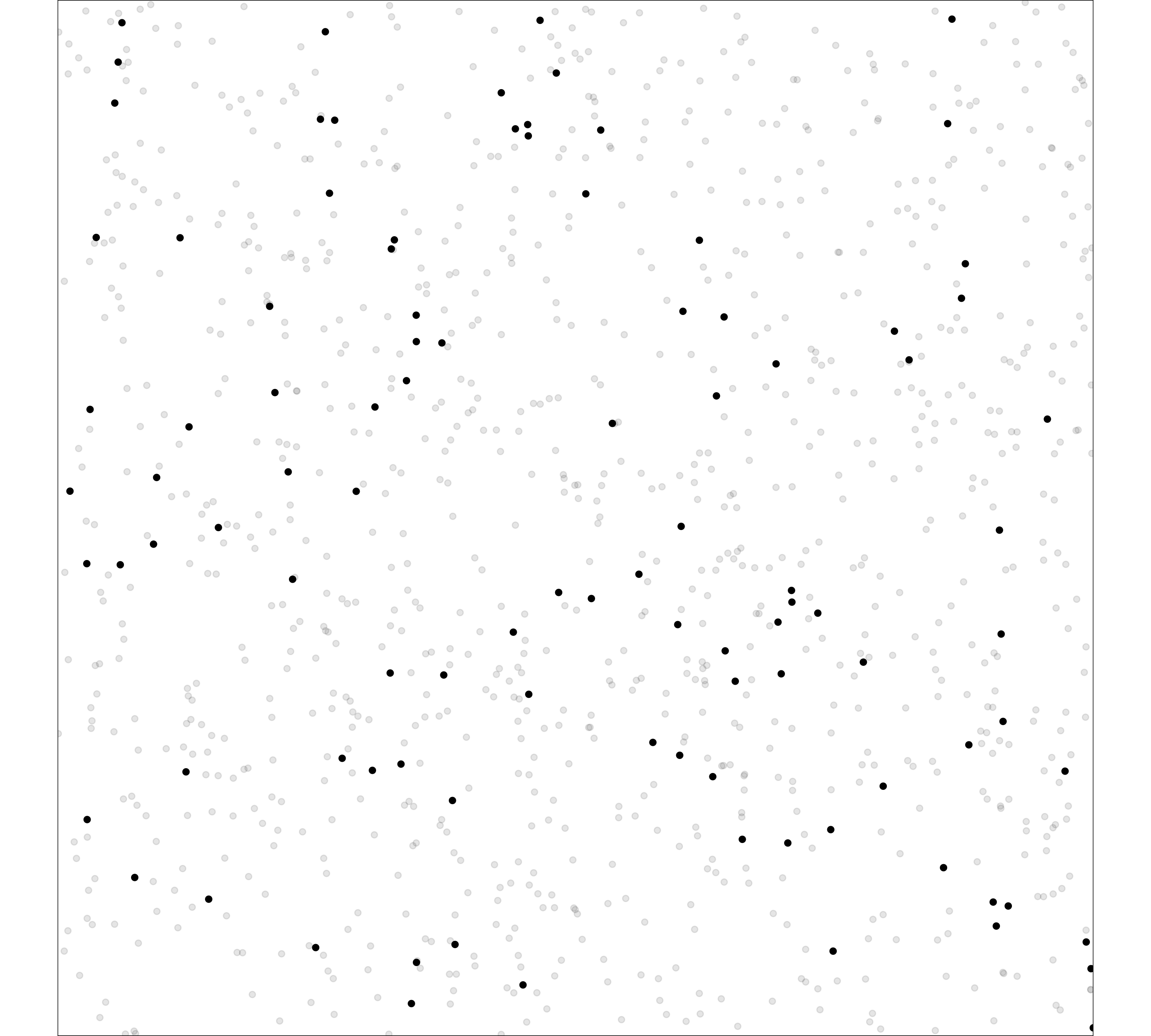
Simple Random
- Only 1 level
- Each observation has same chance of selection
- Sample is often very small relative to population
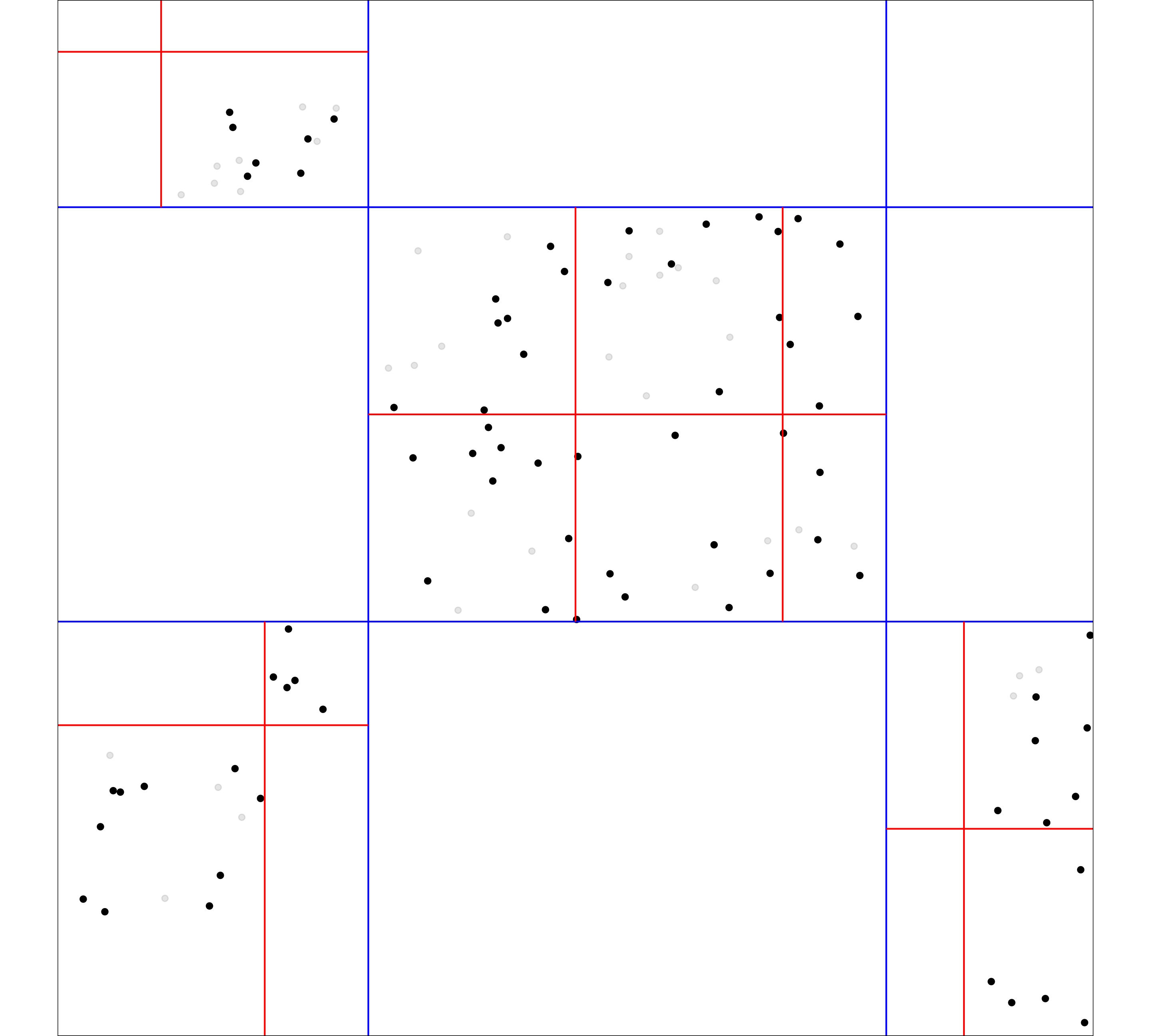
CASPEH
- 3 levels: county, venue, individual
- All sampled without replacement
- Counties and venues sampled with unequal probability
- Individuals sampled with equal probability
- Large fractions of populations sampled
Simple Random
CASPEH

Standard Error Formulas
Simple Random
\[ \sqrt{(1-\frac{n}{N})\frac{variance}{n}} \]
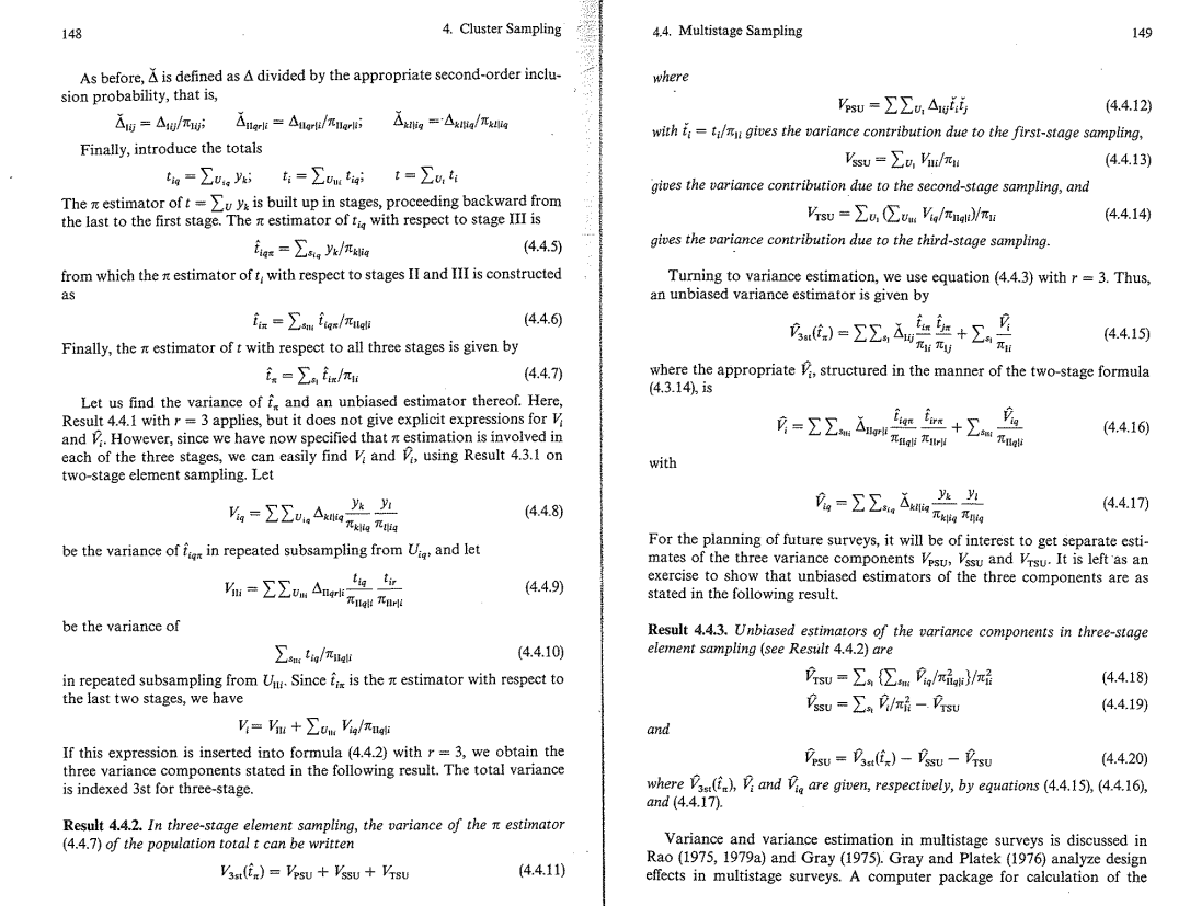
CASPEH

What Are Replicate Weights?
Concepts
- Compute standard errors when formulas are too complicated or inappropriate
- Use the sample as if it is itself a population
- Incorporate sampling design into the calculation of the weights
- Create multiple versions (replicates) of the sample and use variability in those versions for standard errors
- Come in a variety of forms: bootstrap, balanced repeated replication (BRR), jackknife
Bootstrap Resampling
- Draw a new sample from the original sample with replacement using the actual selection probabilities
- Follow the same sampling structure so it’s incorporated into the replicates
- Make an adjustment to the main weights so the replicate resembles the full sample
- Repeat 100 times
Creating Our Replicate Weights
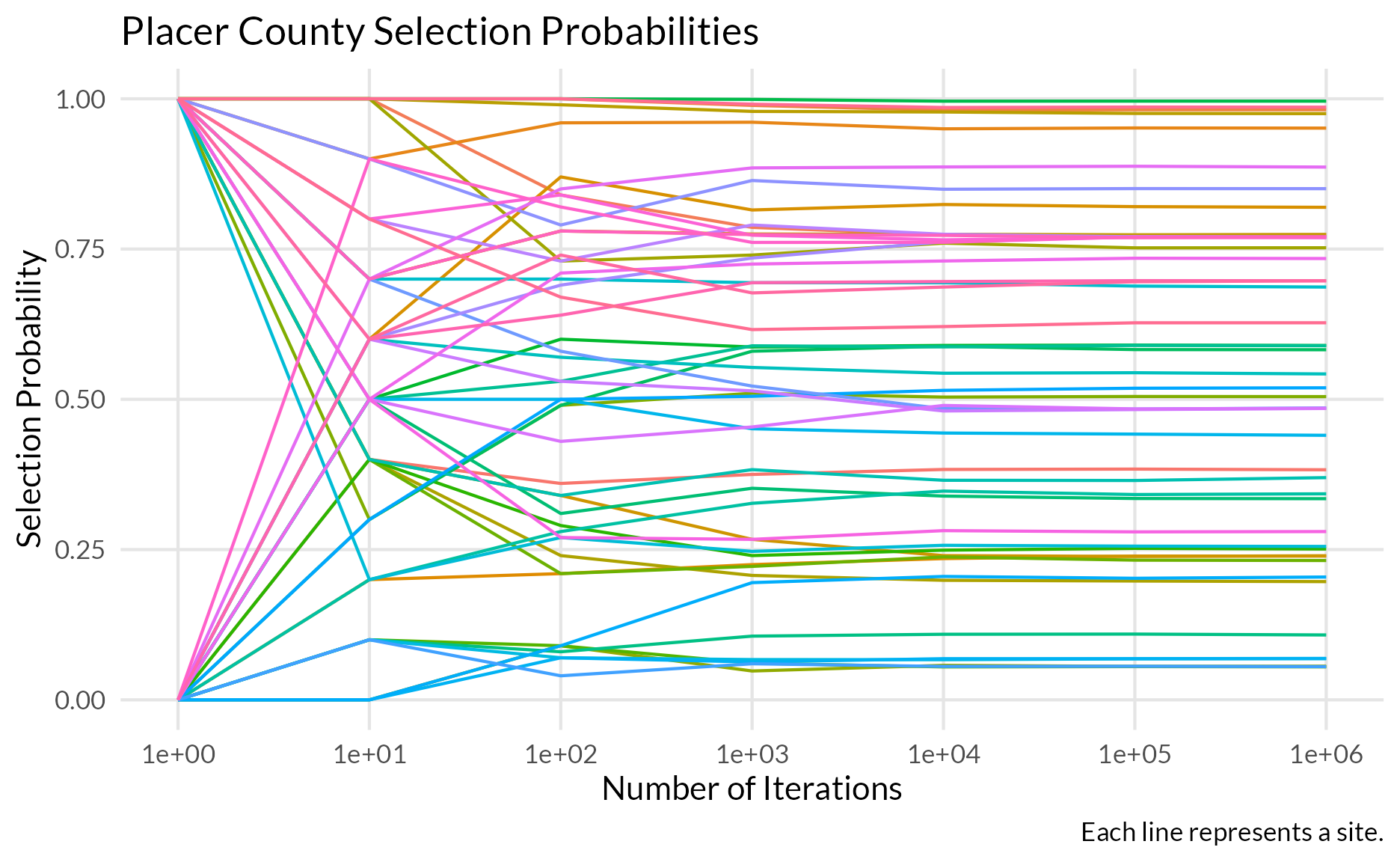
Selection Probabilities
Counties & Venues
- Sampled without replacement and unequal probabilities
- Simulate the sampling procedure many (10,000-100,000) times to get the probability a given county and venue are selected

Individuals
- Simple random sample at venue
- Adjustments for individual non-response
- Adjustments for RDS inclusion
R: Packages
- Relies on
surveyandsvreppackagessurveyis the R workhorse for survey data analysissvrepis the only package which supports multi-stage, unequal probability sampling without replacement and large fractions of population
- Code available on the on-prem (git.ucsf.edu) GitHub
R: Code
design_object <- svydesign(
  ids = ~ county + venue_2 + record_id,
  probs = ~ county_probability + venue_probability + final_individual_probability,
  fpc = ~ county_probability + venue_probability + final_individual_probability,
  pps = "brewer",
  data = design_data
)

options(list(survey.lonely.psu = "adjust", survey.replicates.mse = TRUE))
replicate_weights_design <- as_bootstrap_design(
  design = design_object,
  replicates = 100,
  type = "Rao-Wu-Yue-Beaumont",
  mse = TRUE,
  samp_method_by_stage = c("PPSWOR", "PPSWOR", "SRSWOR")
)
Using Our Replicate Weights
Conceptual Recap
- Estimate statistic of interest using main weights and each set of replicate weights
- Standard error comes from the variability of the replicate estimates with respect to the main weight estimate
R: Data Setup
R: Survey Setup
R: Chi-square Test
R: Regression
Call: svrepdesign.default(ids = ~record_id, weights = ~academic_weight,
    repweights = "academic_rep_weight*", type = "bootstrap",
    mse = TRUE, data = surveys)
Survey bootstrap with 100 replicates and MSE variances.

Call:  svyglm(formula = episode_length ~ race_7cat, survey_object)

Coefficients:
                        (Intercept)                    race_7catNH White
                             40.366                                9.158
                  race_7catNH Black                     race_7catNH AAPI
                             -2.819                               16.096
race_7catNH Native American/Alaskan              race_7catNH Multiracial
                              9.247                               -2.846
                  race_7catNH Other
                             15.916

Degrees of Freedom: 3139 Total (i.e. Null);  93 Residual
  (59 observations deleted due to missingness)
Null Deviance:      11750000
Residual Deviance: 11650000     AIC: 35910
R: Group Means
library(srvyr)

survey_object %>%
  as_survey() %>%
  group_by(race_7cat) %>%
  summarise(survey_mean(episode_length, na.rm = TRUE))
# A tibble: 8 × 3
race_7cat coef `_se`
<fct> <dbl> <dbl>
1 Latinx/Hispanic/Indigenous 40.4 2.50
2 NH White 49.5 3.56
3 NH Black 37.5 3.03
4 NH AAPI 56.5 6.98
5 NH Native American/Alaskan 49.6 5.63
6 NH Multiracial 37.5 2.23
7 NH Other 56.3 15.3
8 <NA> 34.2 5.59Stata: Setup
use "${bhhi_shared_drive}/statewide_survey_processed_data/latest/statewide_survey_processed.dta"

keep if survey_count == 1

svyset _n [pweight=academic_weight], ///
  bsrweight(academic_rep_weight*) ///
  vce(bootstrap) ///
  mse
Sampling weights: academic_weight
VCE: bootstrap
MSE: on
Bootstrap weights: academic_rep_weight_1 .. academic_rep_weight_100
Single unit: missing
Strata 1: <one>
Sampling unit 1: <observations>
FPC 1: <zero>Stata: Regression
(running regress on estimation sample)

Bootstrap replications (100)
----+--- 1 ---+--- 2 ---+--- 3 ---+--- 4 ---+--- 5
..................................................    50
..................................................   100

Survey: Linear regression                         Number of obs   =      3,140
                                                  Population size = 115,572.49
                                                  Replications    =        100
                                                  Wald chi2(6)    =      17.75
                                                  Prob > chi2     =     0.0069
                                                  R-squared       =     0.0078

---------------------------------------------------------------------------------------------
                            |   Observed   Bstrap *
             episode_length | coefficient  std. err.      z    P>|z|     [95% conf. interval]
----------------------------+----------------------------------------------------------------
                  race_7cat |
                  NH White  |   9.157548   4.801016     1.91   0.056    -.2522703    18.56737
                  NH Black  |   -2.81859    4.02318    -0.70   0.484    -10.70388    5.066699
                   NH AAPI  |   16.09569   7.197665     2.24   0.025     1.988528    30.20286
NH Native American/Alaskan  |   9.246603   5.991962     1.54   0.123    -2.497426    20.99063
            NH Multiracial  |  -2.846081   2.898077    -0.98   0.326    -8.526207    2.834045
                  NH Other  |   15.91599    16.3178     0.98   0.329    -16.06631    47.89828
                            |
                      _cons |   40.36602   2.482923    16.26   0.000     35.49958    45.23246
---------------------------------------------------------------------------------------------
Stata: Group Means
(running mean on estimation sample)

Bootstrap replications (100)
----+--- 1 ---+--- 2 ---+--- 3 ---+--- 4 ---+--- 5
..................................................    50
..................................................   100

Survey: Mean estimation                          Number of obs   =      3,140
                                                 Population size = 115,572.49
                                                 Replications    =        100

-----------------------------------------------------------------------------
                            |   Observed   Bstrap *
                            |       mean   std. err.     [95% conf. interval]
----------------------------+------------------------------------------------
 c.episode_length@race_7cat |
Latinx/Hispanic/Indigenous  |   40.36602   2.482923      35.49958    45.23246
                  NH White  |   49.52357   3.537419      42.59036    56.45678
                  NH Black  |   37.54743   3.010734       31.6465    43.44836
                   NH AAPI  |   56.46171    6.94129      42.85703    70.06639
NH Native American/Alaskan  |   49.61262   5.600275      38.63629    60.58896
            NH Multiracial  |   37.51994   2.218442      33.17188    41.86801
                  NH Other  |   56.28201   15.18007      26.52963    86.03439
-----------------------------------------------------------------------------
Questions and Discussion
Additional Resources
- Stata Manual: Bootstrap Replicate Weights
- R
surveyPackage - IPUMS: Replicate Weights in the ACS
- Sharon Lohr: Sampling Design and Analysis
- R
svrepPackage - Beaumont and Emond (2022): A Bootstrap Variance Estimation Method for Multistage Sampling and Two-Phase Sampling When Poisson Sampling Is Used at the Second Phase
- Rao, Wu, Yue (1992): Some Recent Work on Resampling Methods for Complex Surveys

BHHI Methods Meetup Session 1: Replicate Weights